Filter and Sort

You can easily filter and sort large, dynamic datasets in Row Zero. You can apply multiple filters and sorts at the same time. You can also create slicers, which are portable filters that can be moved anywhere in the workbook. Filtering and sorting in Row Zero is similar to Excel, Google Sheets, and other spreadsheets.

Filter

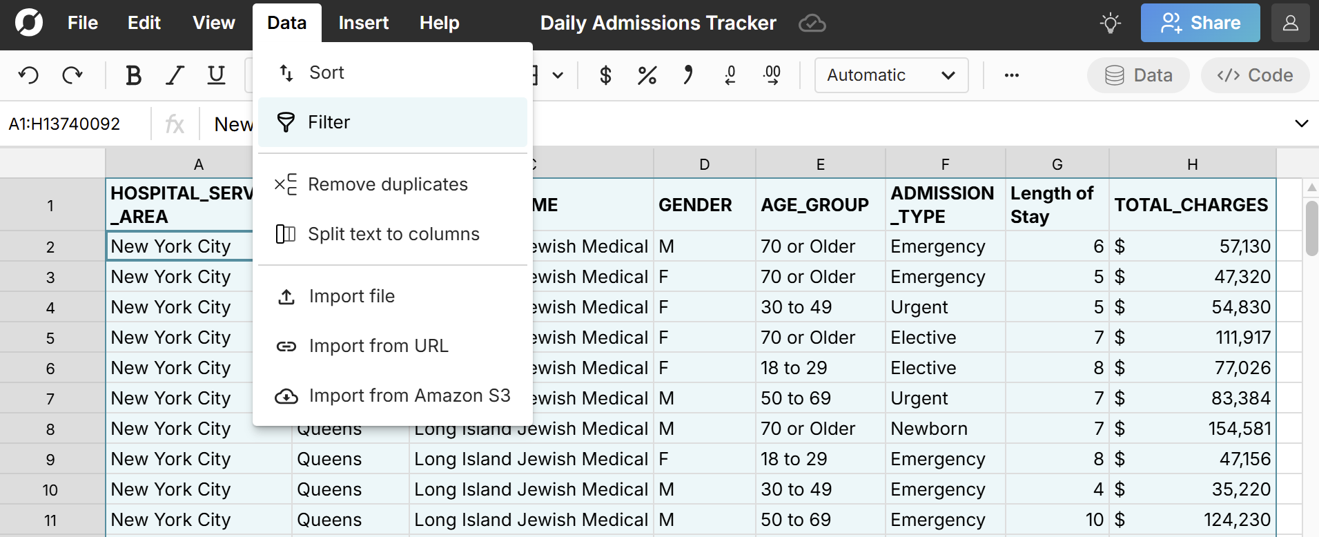
To apply filters a range, select the cells you'd like to filter and go to Data in the header menu and select Filter.

Click the toggle in a column header to sort or filter that column.

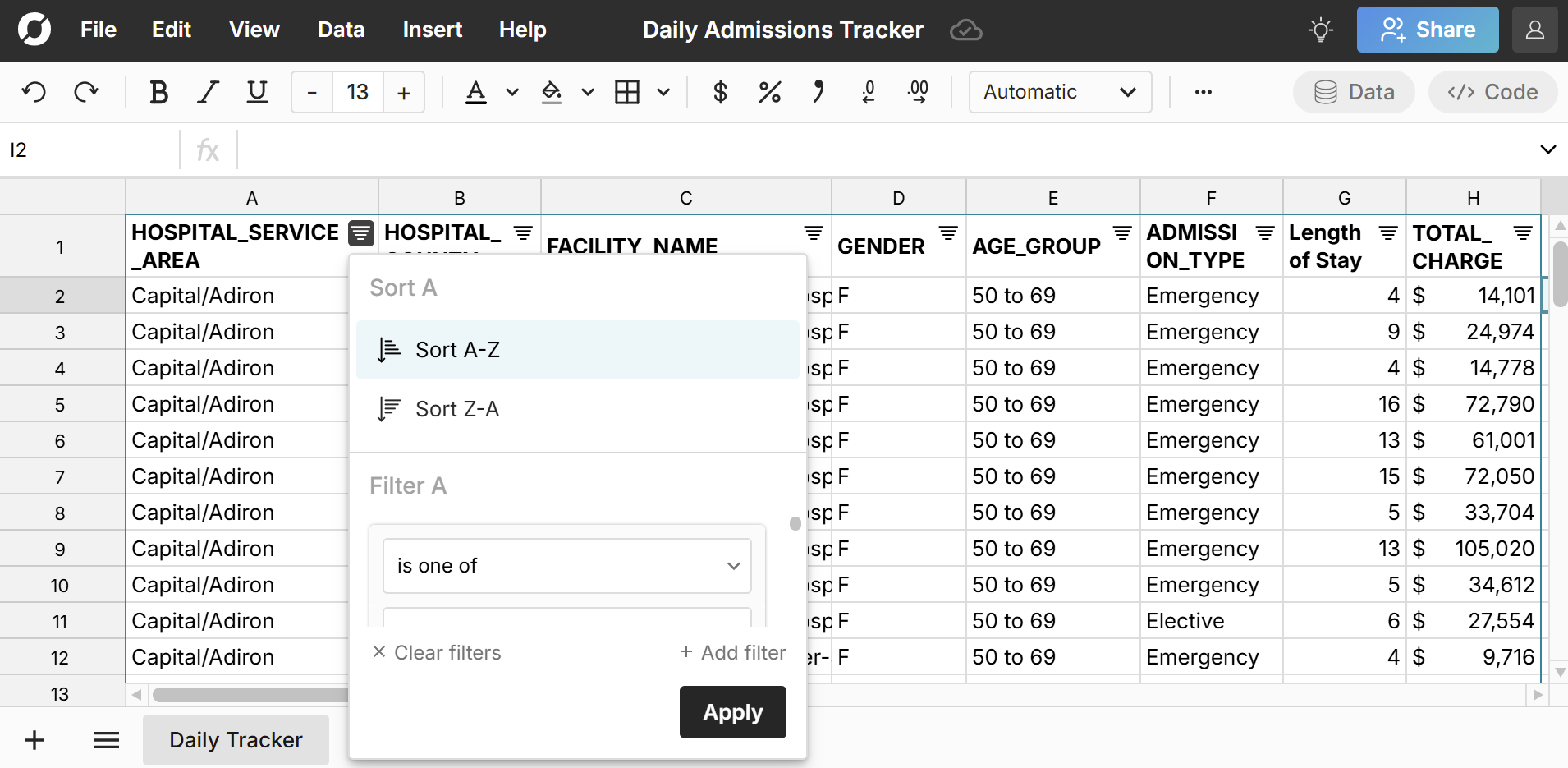
You can filter and sort data tables that same way you filter and sort cell ranges. Data tables are always ready to be filtered, so you don’t need to apply. Just click the toggle in the header column to filter or sort. You can also right-click in the data table and select Sort or Filter.

Filter options

You can apply filters using an evaluation (e.g. greater than 5) or selecting specific values with categorical filtering.

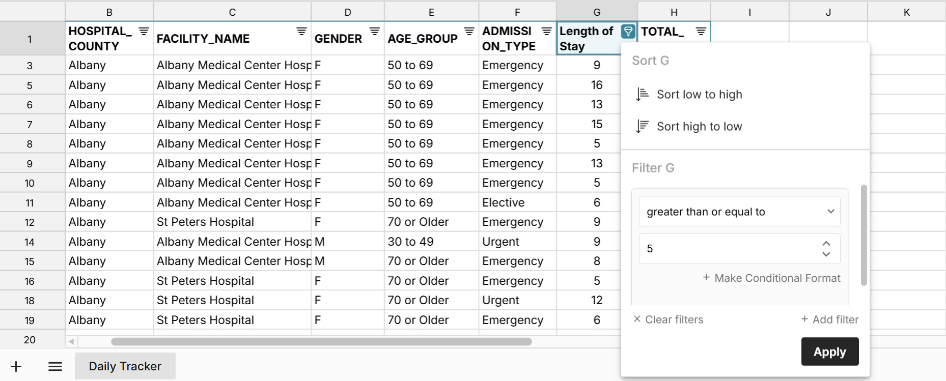
Here are the available filtering options:

• Filter text columns by:
  • is one of
  • contains
  • does not contain
  • starts with
  • ends with
  • is
  • is not
• Filter number columns by:
  • is one of
  • equal to
  • not equal to
  • greater than
  • greater than or equal to
  • less than
  • less than or equal to
• Filter date columns by:
  • is exactly
  • is after
  • is on or after
  • is before

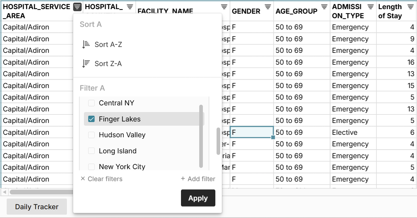
With categorical filtering, you can search for specific values and select one or many values to filter on.

Applying multiple filters

You can apply multiple filters to the same column and also apply filters to multiple columns at the same time. To apply multiple filters to the same column, click the filter icon in the column header and then click + Add filter in the bottom right of the filter dialog to add multiple filters.

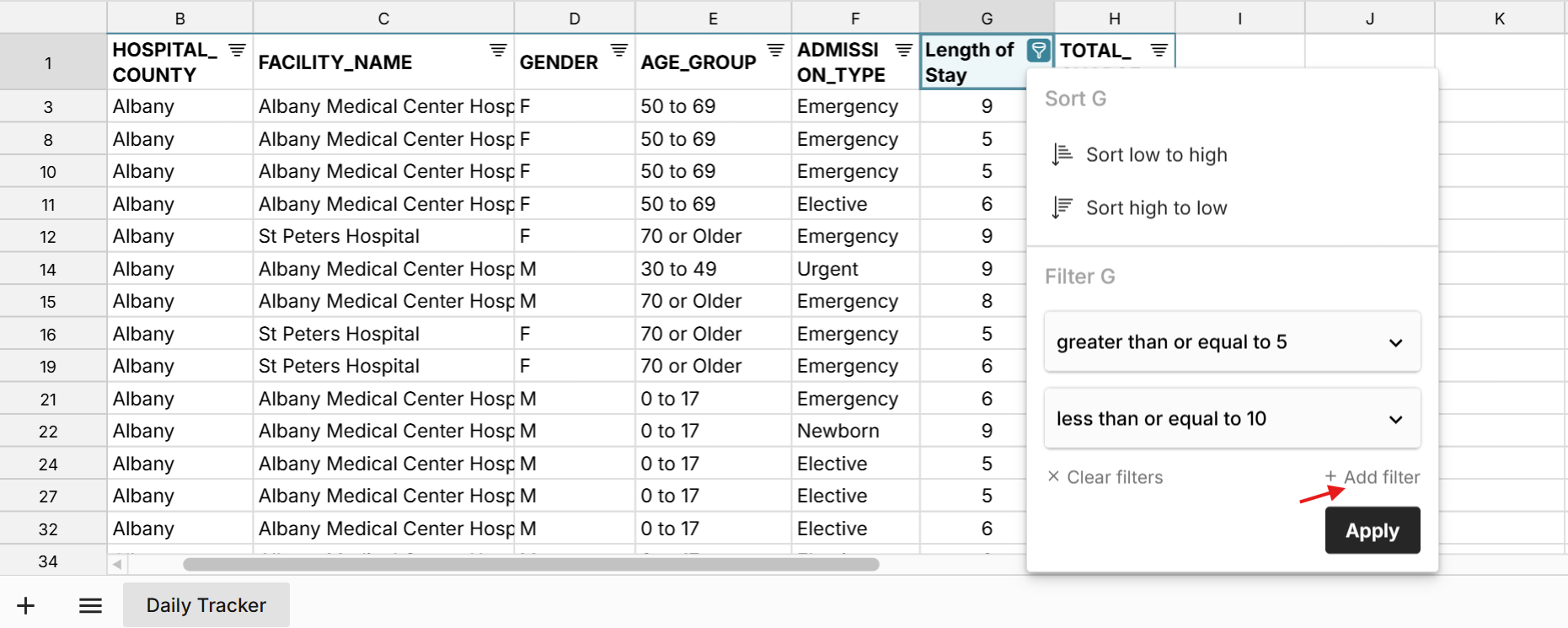
To apply filters to multiple columns, simply navigate to each column and apply filters. Multiple filters are treated as "and" logic, so the sheet will filter to only rows that match all filters.

Convert filter to a conditional format

You can easily make a conditional format from a filter by clicking Make Conditional Format in the filter dialog.

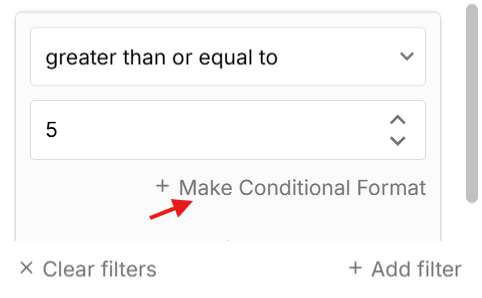
This will open the conditional formatting window with the filter pre-set. Apply formatting and then optionally go back and clear the filter to see the unfiltered data with the previous filter now a conditional format.

Clearing and removing filters

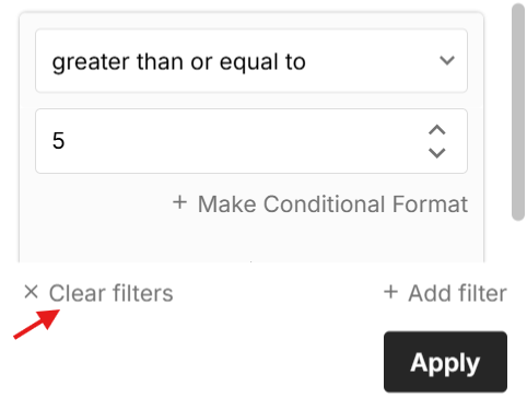
To clear filters, click on the filter icon in the column header and click Clear filters in the bottom left of the filter dialog.

To remove all filters from a range, go to Data in the header menu and select Remove filtered range.

Note that you can only apply filters to one cell range at a time in a sheet. If you want to have multiple filtered datasets on one sheet, use data tables.

Filtering downstream formulas and pivot tables

Using ~ in formulas

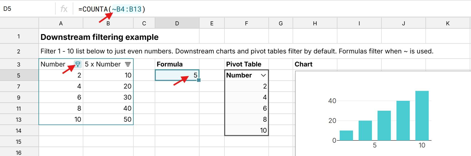
Filtering a cell range or data table does not filter formulas by default. Use the tilde (~) operator immediately before a data table or cell reference if you wish to only operate on the filtered values.

Pivots

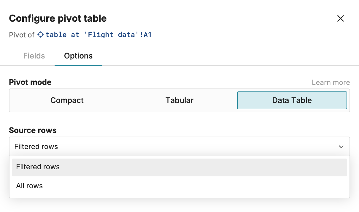
Pivot tables can either use all rows or filtered rows as their source. In the Options tab of the Configure pivot table side pane, select Filtered rows if you would like filters on source data to also filter downstream pivots.

Slicers

Slicers are filters that can be moved anywhere in the workbook. Slicers make it easy to create filters that filter multiple pivot tables and charts at once.

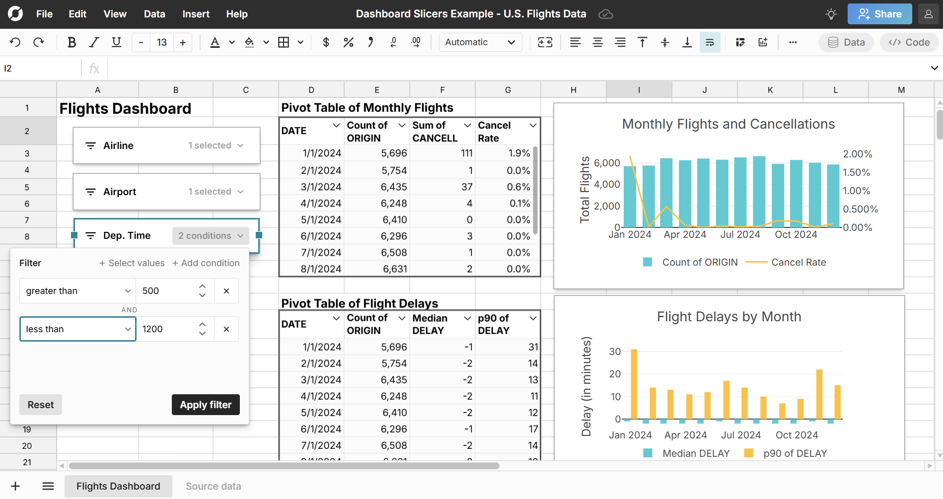
In the example above, pivots were configured to use “Filtered rows” as the source rows, and then slicers were applied to the source data. The slicers were then next to the charts and pivot tables on the “Flights Dashboard” tab to make it easy to filter underlying data on another sheet.

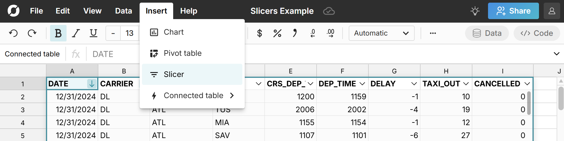
To create a slicer, select your data and go to Insert in the header navigation and select Slicer.

Sort

There are two ways to sort cell ranges in Row Zero:

1. Using the Filter dialog: See Filter above.
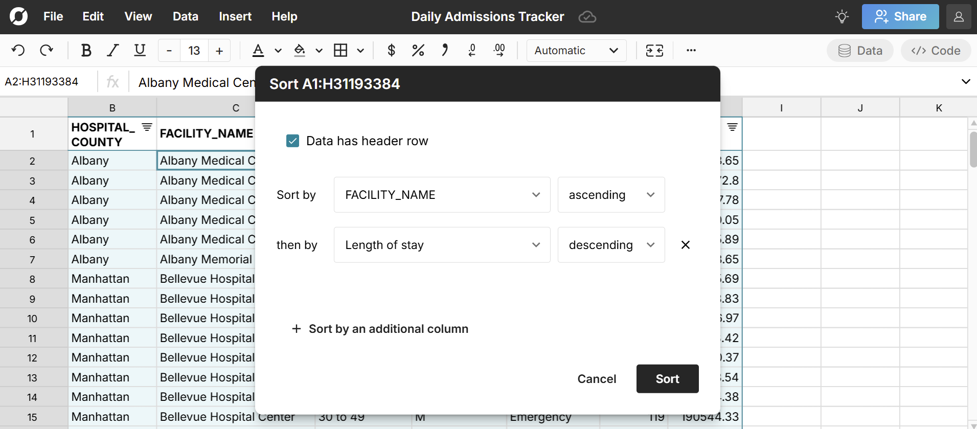
2. Using the Sort dialog: Go to Data in the header menu and select Sort. This menu an also be accessed or by right-clicking on selected data and selecting Sort range.

If needed, you can sort multiple columns.

Sort by color

You can sort by color via the filter dialog. Sort by color lets you pull rows with the same color to the top of the workbook for review. This is particularly powerful when combined with conditional formatting that automatically color-codes your data.