Pivot Tables in Row Zero

Pivot tables make it easy to summarize, analyze, and explore large datasets. Row Zero pivot tables are dynamic and automatically update as source data changes. There are three pivot modes:

Compact: Best for final presentation of data. Supports nesting fields, collapsible groupings, and subtotals.
Tabular: Best for detailed tables. Shows row fields in separate columns, repeated labels, and bottom subtotals.
Data table: Best for transforming data and creating charts. Supports computed columns, filtering, and sorting.

The documentation below shows how to create and work with pivot tables in Row Zero.

Configure pivot tables

Create a pivot table

You can create pivot tables from both cell ranges and data tables. Here's how:

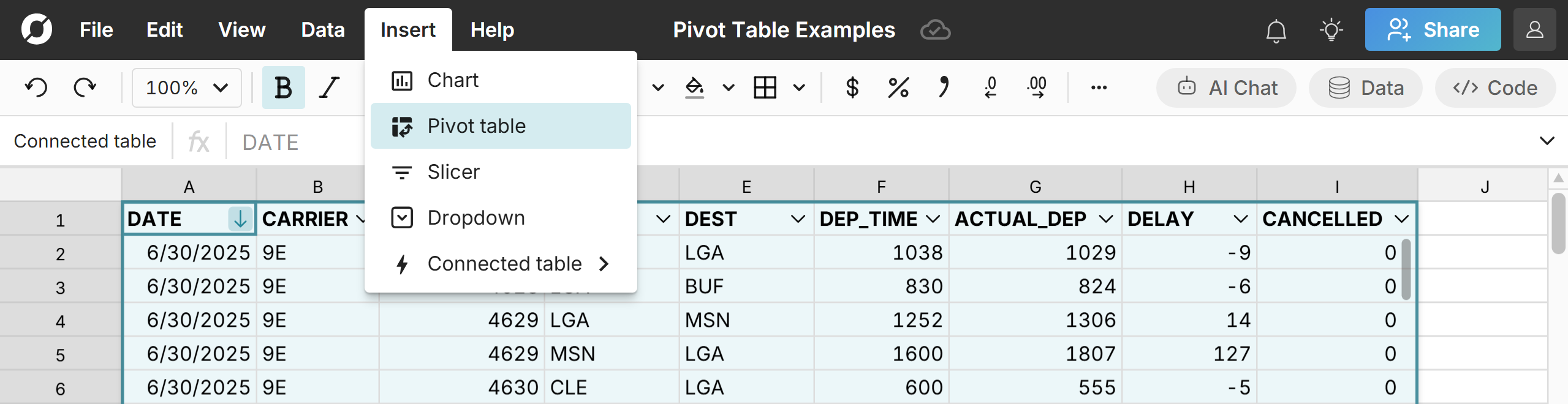
Select the data you want to create a pivot table from, go to Insert > Pivot table. You can also right-click on a cell in a data table or a selected cell range and select Pivot, or use a keyboard shortcut to insert a pivot table (Alt, N, V on Windows or Option, N, V on Mac).
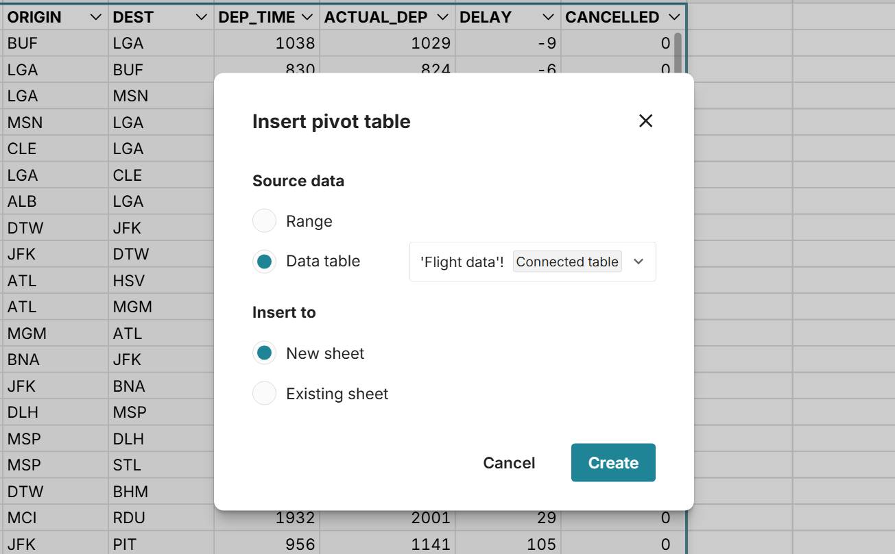
Select your pivot table location. You can insert to a new sheet or a specific cell on an existing sheet.
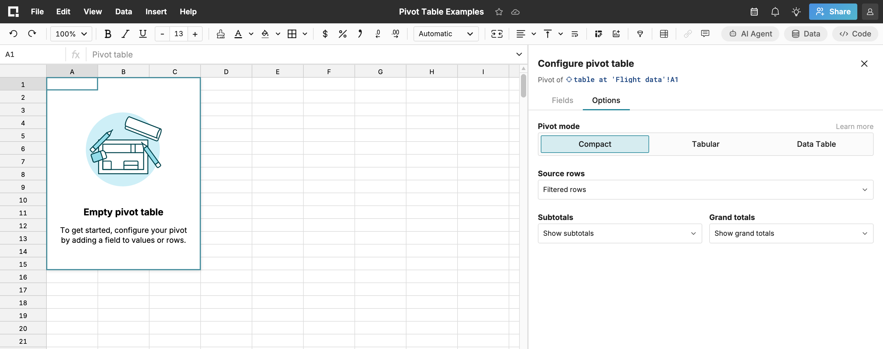
An empty pivot table will be created.
Click Options to choose your pivot type (Compact, Tabular, or Data Table), whether source data includes filtered or all rows, and subtotal options.
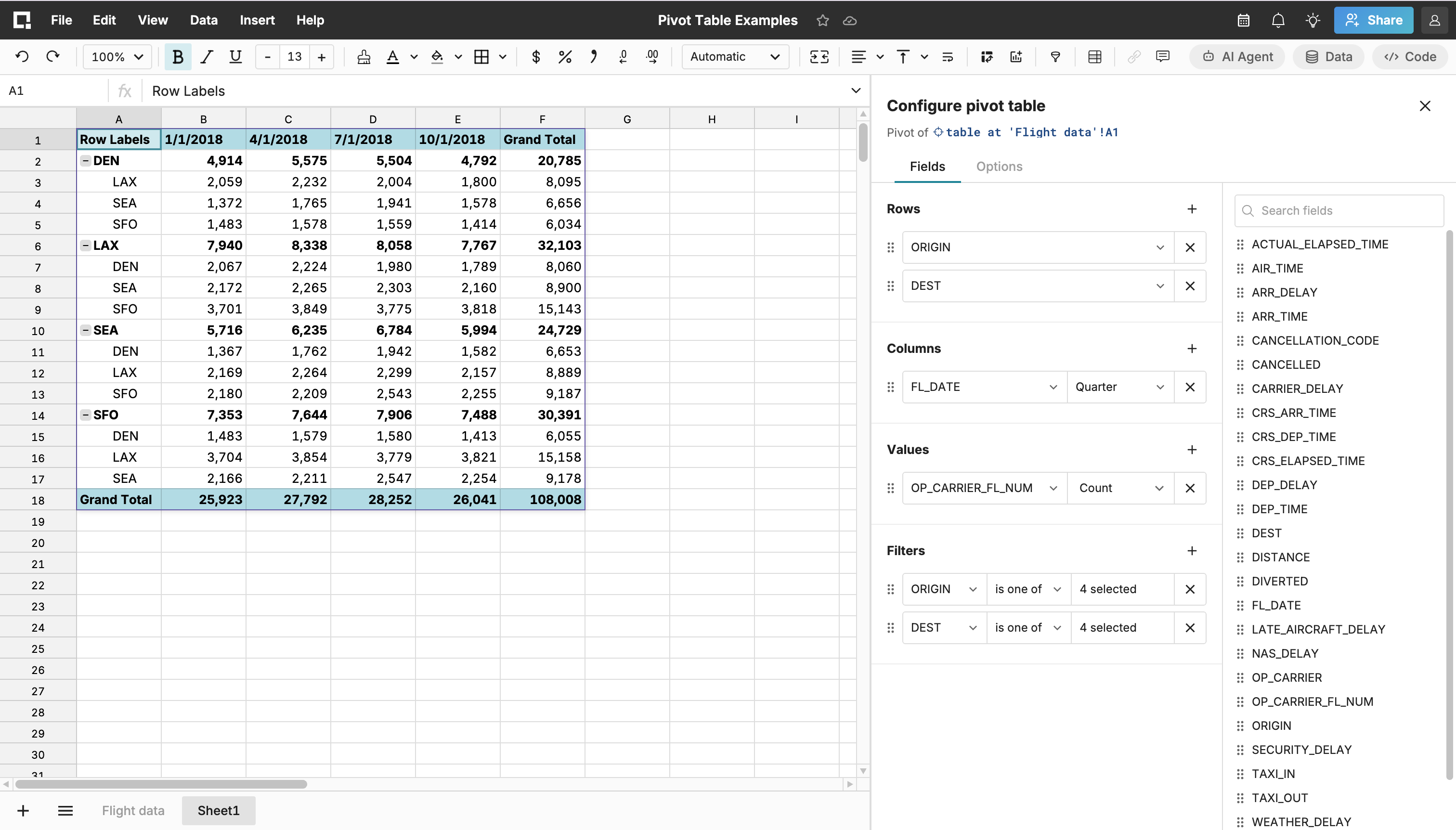
Click Fields to configure your Rows, Columns, Values, and Filters in your pivot table.
- Rows and Columns: Think of these as "a row for each" or "a column for each" of whatever field you choose. Rows and columns are optional, but it is more common to use Rows. If you select multiple fields, they’ll be nested in groupings.
- Values: Values are the fields you want to calculate. See options for Value calculations below.
- Filters: Filters the source data used in the pivot table. Pivot table filters support the full suite of filter options.

Here's an example pivot table that summarizes a dataset of 25 million U.S. flights with Rows grouped by Origin and Destination, Columns grouped by year, and Values for Count of flights (by year). Filters are also added to limit to flights in and out of DEN, LAX, ORD, SEA, SFO.

Value calculations

You can set Values as Columns or Rows. Values have the following built-in calculations:

Average - Average across values for each row/column grouping
Count - Counts the number of values for each row/column grouping
Count unique- Counts the number of unique values for each row/column grouping
First - First instance of a value for each row/column grouping
Last - Last instance of a value for each row/column grouping
Max - Maximum value for each row/column grouping
Median - Median value for each row/column grouping
Min - Minimum value for each row/column grouping
Percentiles - Lets you specify a percentile value to return for each row/column grouping. Percentile options include 10, 25, 50, 75, 90, 95, 99, 99.9.
Std dev - Standard deviation of values for each row/column grouping
Sum - Sum of all values for each row/column grouping
Variance - Variance of values for each row/column grouping

Group date fields in rows or columns

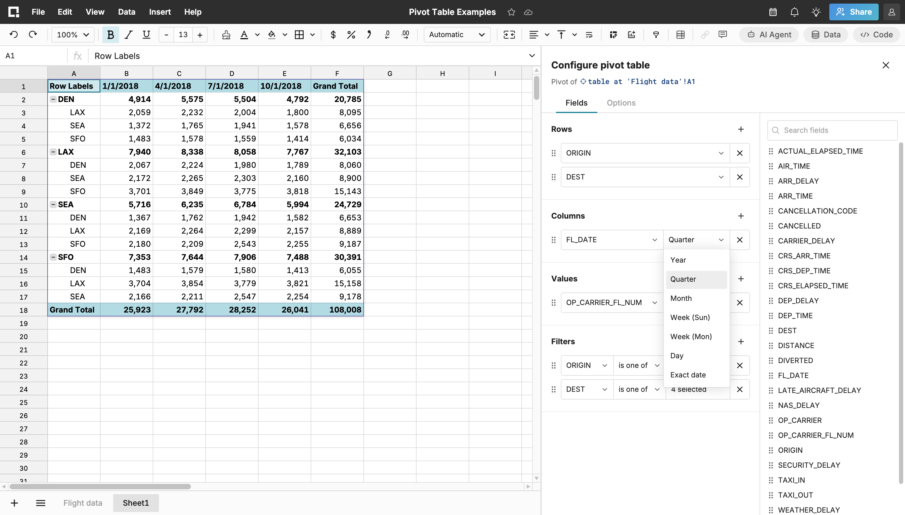
Pivot tables have built-in date grouping. You can group date fields in rows or columns as seconds, minutes, hours, days, weeks, months, quarters, or years. Below, we update the date grouping from year to month in our pivot table above.

Edit and update pivot tables

Pivot tables dynamically update as source data changes. If you edit, add, or delete source data, your pivot table updates automatically.

To edit a pivot table, right-click on the table and select Edit pivot table. Pivot tables dynamically change as you make edits.

Move, copy, and delete pivot tables

You can drag pivot tables around a sheet or cut/copy and paste to another sheet. To cut/copy a pivot table, right-click on the top-left cell in a pivot table and select 'Cut' or 'Copy' and then use 'Ctrl + V' to paste. To delete a pivot table, click in the top-left cell of the pivot table and use your delete key.

Slicers

Slicers are filters that can be moved anywhere in the workbook. If you have selected Filtered rows as your Source rows, you can use slicers on your source data to filter your pivot table. To use slicers to filter a pivot:

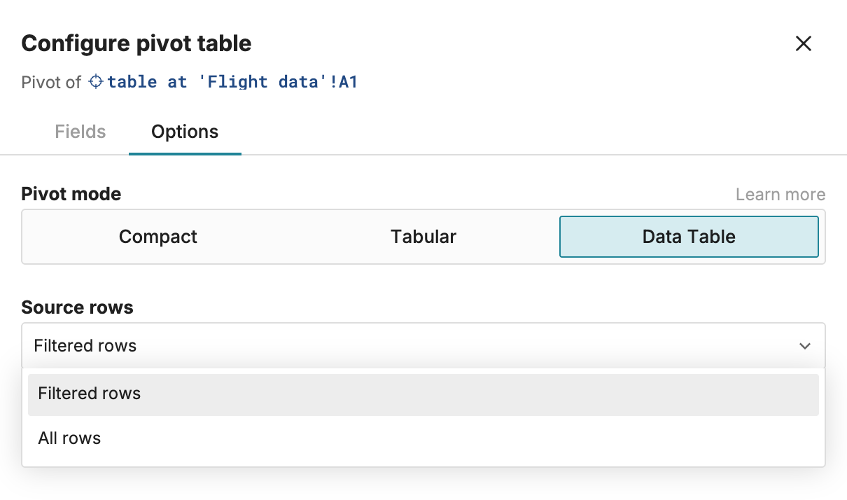
In the Configure pivot table window, select Filtered rows in the Source rows dropdown menu.
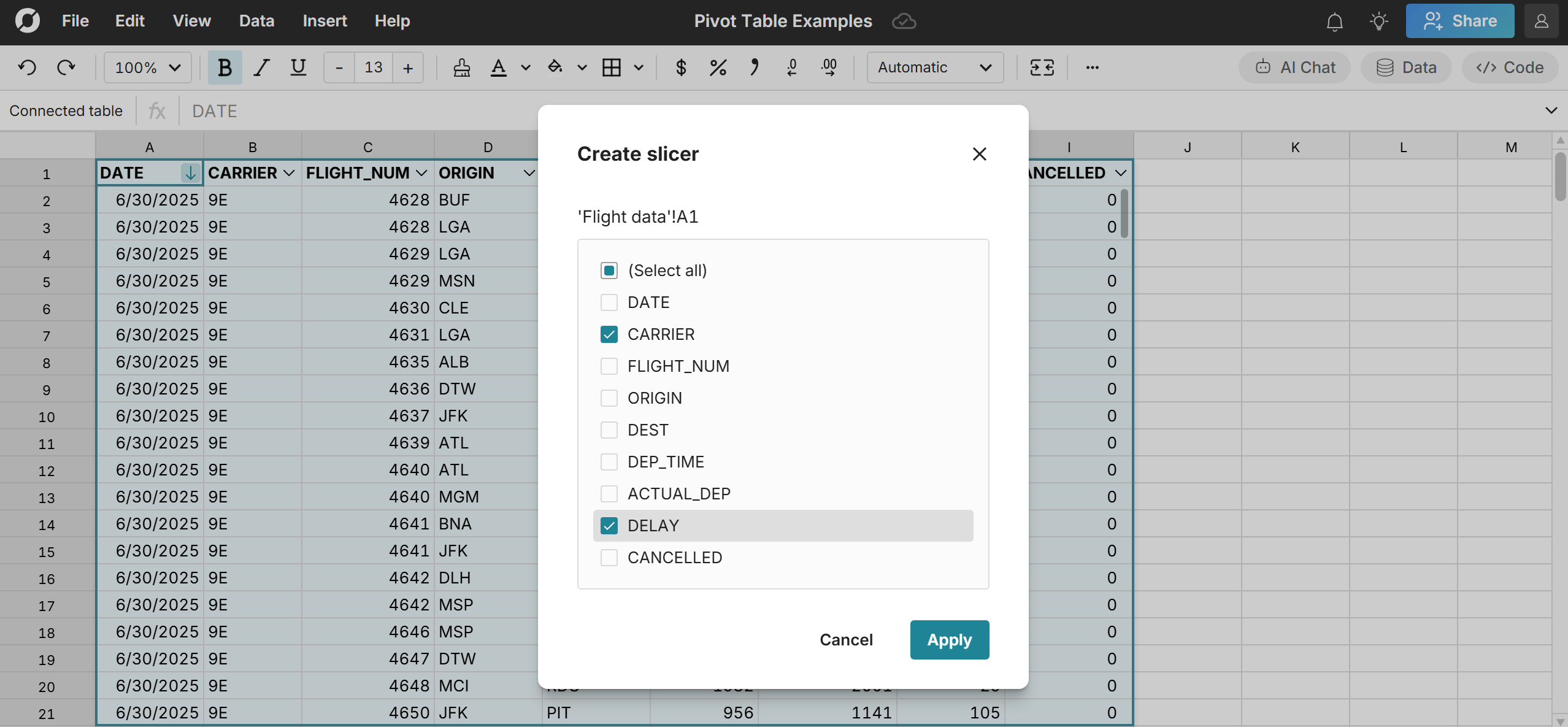
Click a cell in your pivot table's source data and go to Insert > Slicer. Select the slicer columns and click Apply.
A slicer is created for each column selected, which you can move or cut/paste around your workbook.
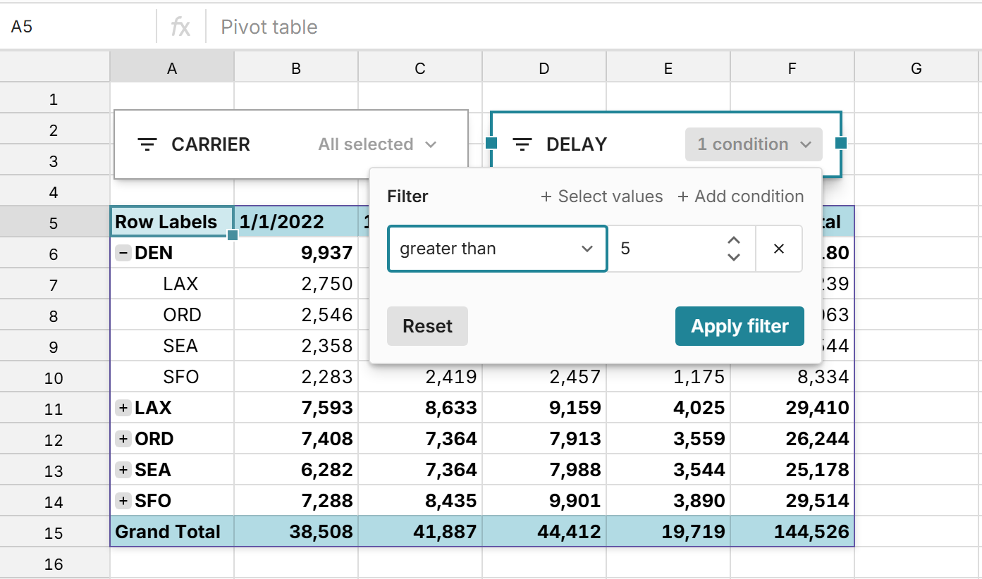
Click the slicer dropdown to open the filter. You can select from the list of values, search for a value, or filter by one or more conditions (e.g. >=5). Click Apply and the source data will filter accordingly. The pivot table dynamically updates to reflect the filters applied to the source data. See Slicers to learn more.

Compact and Tabular mode

Sort

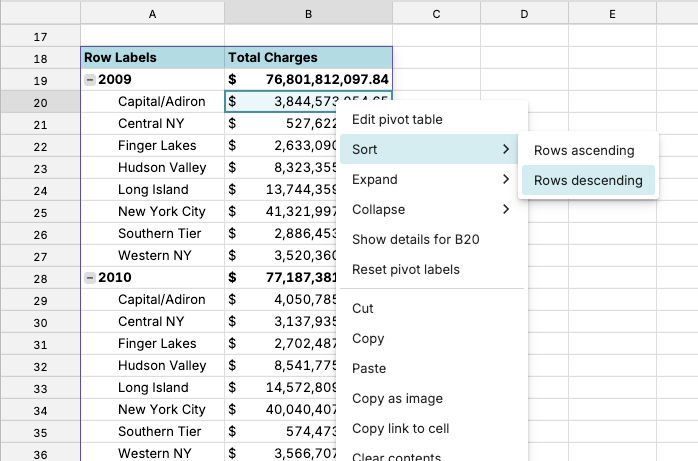
Sort a compact or tabular pivot table on any row or column field, in ascending or descending order. You can sort on labels, values, and totals.

To sort a pivot table in tabular or compact mode:

In the pivot table, right-click the label, value, or total you want to sort on.
Select Sort, then choose a sort order.

If the pivot uses aliases, sort will operate on the aliases rather than the original value.

Sorting on a nested field sorts within its grouping. In the example below, sorting on a region would sort the regions within each year. The year order would stay the same.

Reference pivot table data in formulas

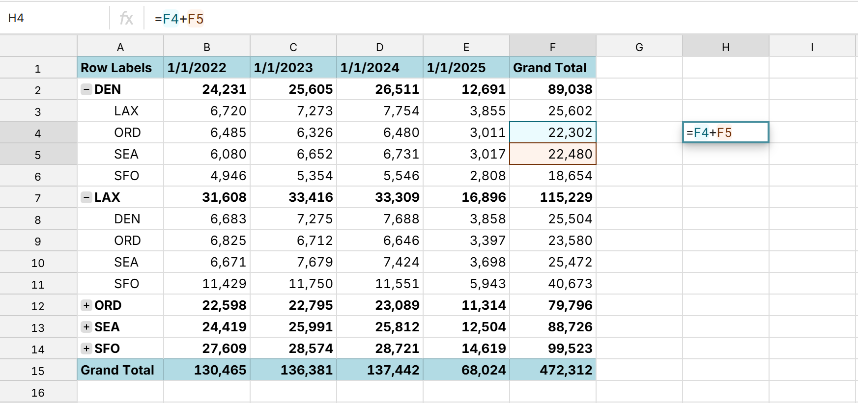
Compact and Tabular mode support cell references, so you can easily reference any cell in a pivot table in downstream formulas.

Formats in Compact and Tabular mode

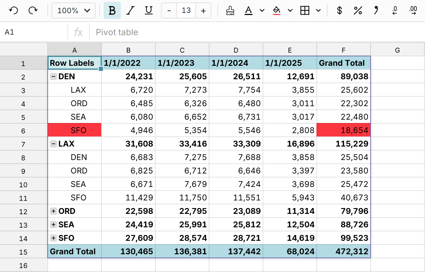
Compact and Tabular mode pivot tables also allow you to format specific cells in the table. Select the cell(s) you would like to format, and then select the desired formatting options in the tool bar.

Add aliases for column or row labels

You can also add aliases for pivot table row and column labels in standard mode. To add an alias, click on the cell and type the alias. To clear aliases, right click and select Reset pivot labels.

Data table mode

Data table mode offers advanced features for transforming data. You filter, sort, chart, and add computed columns to the pivot table.

You can switch to data table mode by selecting Data table as your Pivot mode.

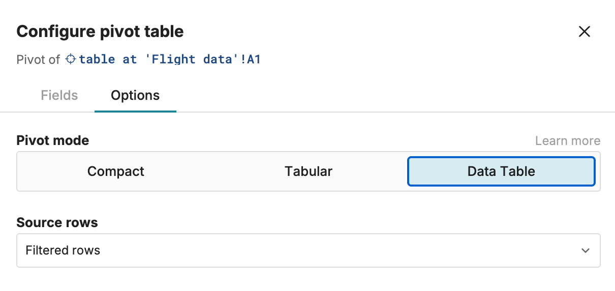
Note: Data table mode does not support nested groupings, subtotals, or cell references. You’ll need to switch to Compact or Tabular mode for those features.

Filter and sort

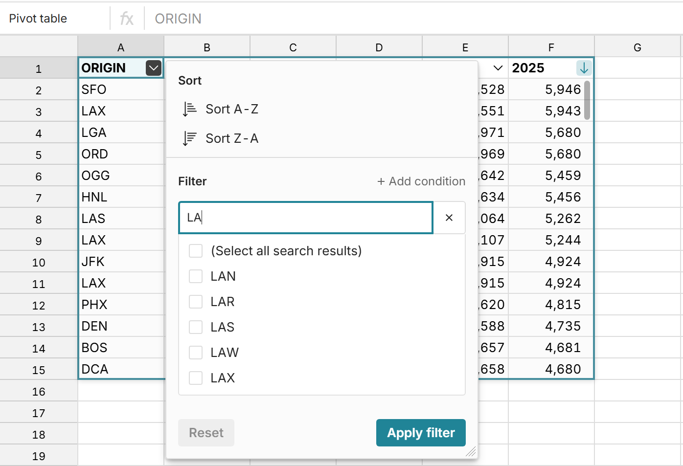
Pivot tables in Data table mode have built-in filtering and sorting. Click the down arrow in a column header to sort or filter your pivot table.

Create charts from data table pivots

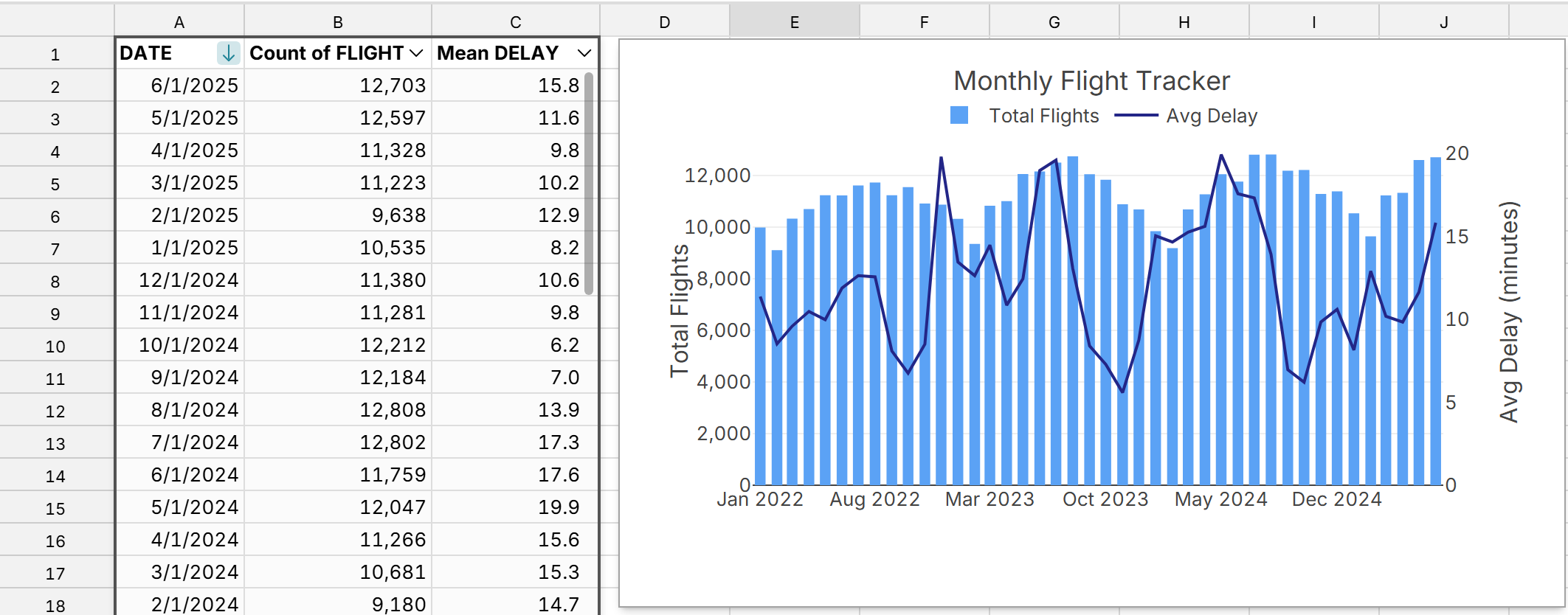
To create a chart from a pivot table in Data table mode, select a cell in each pivot table column to include in your chart and go to Insert > Chart in the header navigation. Charts built from pivot tables update dynamically in sync with the pivot table, as the pivot table changes or is updated with new data. See Charts to learn more.

Add computed columns to data table pivots

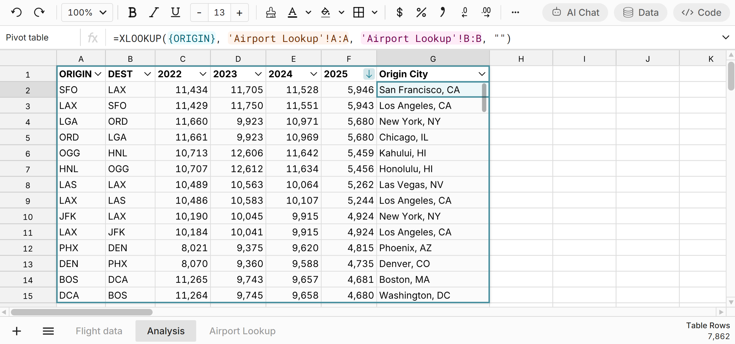
To add a computed column to your pivot table, write a formula in the first column to the right of the pivot table and reference a pivot table column in the formula. The formula dynamically fills in every row in the column with the formula applied. See Data tables for more information about computed columns.

Formats in data table mode

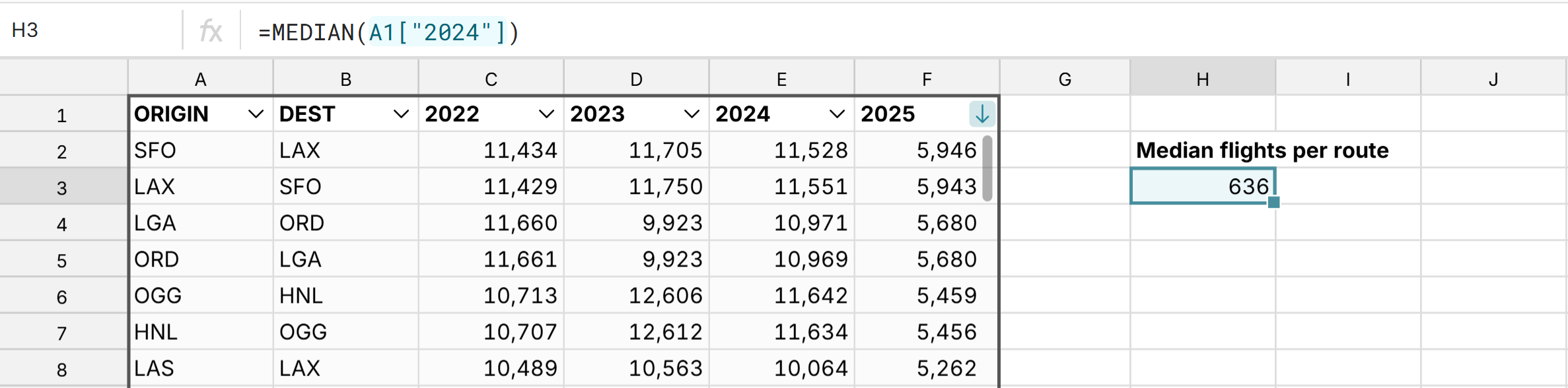
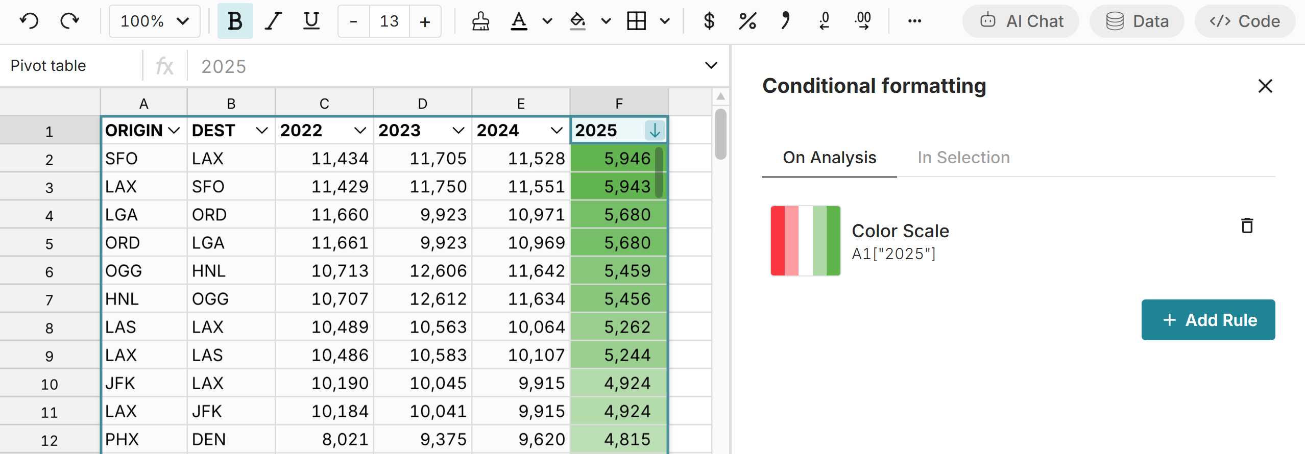
In Data table mode, you can reference pivot table columns in formulas using the cell location of the top-left corner of the pivot table and the column name. In the example below, the pivot table starts in cell A1 and has a column named "2024". To use this in a formula, use A1["2024"], which you can see in the example below.

You can also apply any formatting to your pivot table but formatting is applied to the entire column when in Data table mode.

To hide pivot table columns in Data table mode, right-click on the pivot table and select 'Manage columns' and unselect whatever columns you'd like to hide.

On this page